Decontaminating amplicon sequencing data for the drinking water microbiome

Summary

Decontaminating low biomass microbiome data is crucial, especially in the drinking water microbiome field. I think creativity and transparency in our approaches will be critical to approaching this ongoing challenge. Below, I summarize my experiences analyzing contaminated amplicon data. In a future post, I’ll focus on metagenomics.

Why write about data decontamination?

• To share what I’ve learned and to stimulate discussion on how to improve decontamination for drinking water microbiome research.
• Because I felt like I was mostly alone with this and maybe you too are struggling with some contaminated data right now (though I hope not!).
• To show my mistakes. It is okay to make mistakes in science, just don’t keep them to yourself.
• Distraction from COVID-19, the ultimate contaminant of today.

For a limited collection of resources on this topic, skip to the References section at the end.

Why is decontamination essential (and hard) with low biomass samples?

The golden rule of systematic contamination in microbiome data is this: The less DNA in the sample, the higher the fraction of total DNA that comes from contamination (Salter et al. 2014). Said another way, in low biomass samples, the signal to noise ratio of sample to contaminants is low. Sources of contamination in microbiome studies include 1) reagents and materials used to extract and amplify DNA, 2) the sampling and laboratory environments, and 3) other samples processed at the same time as low-biomass samples.

I study highly purified water, which has very low cell counts (as low as 100 cells / mL). Even with good collection methods, low biomass is still an issue. To make matters more complicated, the water used to make reagents also undergoes purification, meaning it might contain similar microorganisms to the ones I am trying to study. This means decontamination is critical.

The first try, or the story of some messy data

Before 2017, I had never worked with low-biomass microbiome data. I had been lucky enough to choose systems for study that had dense biomass. Then I entered the field of potable reuse, where I study treated wastewater as it passes through stages of advanced treatment. This means my samples range from high (1E7 cells / mL) to low (1E2 cells / mL) biomass, which led to contamination issues in our lab’s first microbiome study (Kantor et al. 2019). Samples we had taken of reverse osmosis (RO) permeate had almost nothing in them, while our treated wastewater samples had inhibitors. It was nearly impossible to extract DNA from granular activated carbon samples using any of the kits we had in the lab. We made a lot of mistakes in that first project, from which followed an agonizing year of analyzing contaminated data.

When we got back the 16S rRNA gene (V4) amplicon sequencing results, the first thing I noticed was the low quality. Digging deeper, I discovered a single amplicon sequence variant (ASV) had taken over the dataset, resulting in homogeneous reads (hence the low quality). After removing this ASV, there were still other sequences present in our filter blanks and amplification negative controls and widespread across samples. I tried subtracting all negative control ASVs from the samples, but that removed most of the data. After plotting heatmaps, I realized our high-biomass samples had contaminated some of the low-biomass samples, including negative controls.

This contamination made me question all of my data, and everyone else’s. Many papers I read said they had so few reads in their negative controls that they just ignored the controls altogether and threw out other low read-count samples. We had used a Speedvac to concentrate gDNA and amplicons, which had concentrated our contaminants in both samples and controls. Hence, some controls and low-biomass samples had high read-counts, so removing samples by read-count didn’t make sense. My literature searches at that time turned up Salter et al. (2014), and just a few others discussing the “kit-ome”. Midway through my analysis, the decontam R package was released (Davis et al. 2018). To my dismay, it didn’t identify even the most visually obvious contamination (maybe because the SpeedVac messed with our DNA concentrations). I opted to present my controls alongside my samples and to remove only the most egregious contaminants.

Not surprisingly, reviewers were suspicious of the data, just as I was. At their suggestion, I tried using differential abundance for decontamination. I began with the assumption that every ASV present in the controls was a contaminant until proven otherwise. I used the R package DESeq2 to analyze ASVs present in both samples and controls. I kept ASVs that were significantly enriched in samples over controls and ASVs found only in samples. The results of this approach lined up with visual decontamination. The paper passed review and I posted my extensively commented Jupyter notebooks on Github (https://github.com/rosekantor/16S_metagenomics_notebooks).

The same year our study came out, some good papers on contamination in microbiome studies were published (Karstens et al. 2019; Eisenhofer et al. 2019). I also found a few that had been written after I’d finished the decontamination steps of my study (de Goffau et al. 2018 and this blog post from the Fierer Lab.)

The second try: eyes on the data

In our next study, we filtered larger volumes (using dead end ultrafiltration and PEG flocculation), we were even more careful with sample handling, and we included more controls (filter/flocculation negative controls, extraction positive and negative controls, amplification positive and negative controls). Our biggest challenge was that this time, we wanted to use the same DNA extraction protocol for all samples, including high-biomass tertiary wastewater and low-biomass RO-permeate. We tested 3 different kits with and without multiple modifications, we consulted with technical support from the kit manufacturers, and optimized our method. To prevent contamination, we separated pre- and post-PCR steps spatially and temporally, we batched extractions by low vs. high biomass and sample site, and we got brand new multichannels that didn’t require us to bang tips on and pull tips off.

In spite of this, the golden rule of contamination still holds. Low biomass samples have high contamination. While we filtered a lot more water this time (up to 4000 L of RO permeate), we could use only 200 ul of a 3 mL flocculation pellet per DNA extraction, resulting in low gDNA concentrations. In the data, there are 185 ASVs in at least one sample AND one negative control. Below, I’ll show analysis for some of the most abundant of these ASVs.

Controls we have:

• Positive gDNA mock community controls (Zymobiomics)
• Positive extraction mock community controls (Zymobiomics)
• Field negative controls that underwent filtration and flocculation
• Extraction negative controls

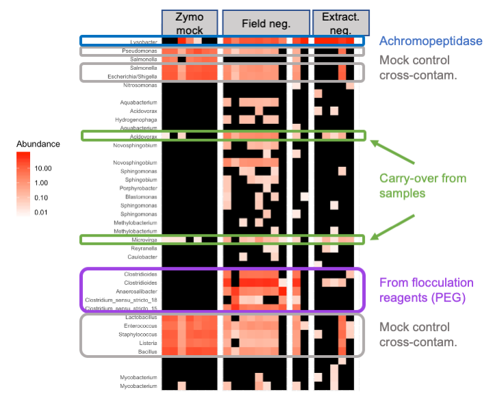
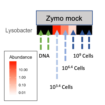
First, in all extraction negative controls and some positive controls, Lysobacter enzymogenes is at high relative abundance. This is the bacterial source of achromopeptidase used in our extractions (Fig. 1, blue). Zooming in on this ASV in the positive controls (Fig. 2), we see that the relative abundance of Lysobacter depended on how many cells from the mock community (Zymobiomics community standard) were added to the extraction controls, and Lysobacter is absent from the DNA-only amplification controls (Zymobiomics DNA community standard).

Second, looking into the field negative controls, which include filtered-flocculated and flocculated-only samples, we see a group of Clostridiales that likely came from the PEG used in flocculation (Fig 1, purple). In the last field negative control a new bottle of PEG was used, and these ASVs are absent.

Third, the mock community has cross-contaminated into the field negative controls (Fig. 1, gray), which suggests other sample cross-contamination may also have occurred (Fig. 1, green). Since we batched extractions by sample location instead of randomizing them, hopefully cross-location contamination is limited.

Figure 1. Looking at the most abundant ASVs that are present in at least one control and one sample. Heatmap made with Phyloseq.

Figure 2. Lysobacter ASV in positive controls. Heatmap made with Phyloseq.

As with the first dataset, published methods for data decontamination failed to pick up all the major contaminants I knew were present by visual inspection (there is still plenty of room for new statistical methods in this field!). My rigorous decontamination method with DESeq2 removed some important ASVs from high-biomass samples that had cross-contaminated into controls. This happened because these ASVs were from tertiary wastewater, and weren’t present in enough of the other samples to be statistically significantly enriched in samples over controls. To get around this, I opted to group samples by location and compare each group to the full set of controls, identifying ASVs that were significantly enriched in that sample location as “true” ASVs. The full “true” set included all ASVs that were “true” in any sample type and ASVs not found in any control.

Conclusion

The decontamination process has underscored for me how important it is to have one’s eyes on the data, to play with the data, and to test both published and new methods on the data. As with most sequencing-based bioinformatics, but especially with decontamination, there is no out-of-the box solution that will work for every dataset. I think exploration and creativity are essential to science, even if we are sometimes taught that they are “unscientific”. In publications, we only see the final results, but the process behind them is sometimes oversimplified. The risk here is that labs taking up microbiome work for the first time will assume that the work is as easy as copying someone else’s methods. Sharing what happens behind the scenes takes guts, and I hope we can encourage each other to do this more often. It is important for advancing our field.

References

Davis, N. M., Proctor, D. M., Holmes, S. P., Relman, D. A., & Callahan, B. J. (2018). Simple statistical identification and removal of contaminant sequences in marker-gene and metagenomics data. Microbiome, 6(1), 1–14. http://doi.org/10.1186/s40168-018-0605-2

Eisenhofer, R., Minich, J. J., Marotz, C., Cooper, A., Knight, R., & Weyrich, L. S. (2019). Contamination in Low Microbial Biomass Microbiome Studies: Issues and Recommendations. Trends in Microbiology, 27(2), 105–117. http://doi.org/10.1016/j.tim.2018.11.003

de Goffau, M. C., Lager, S., Salter, S. J., Wagner, J., Kronbichler, A., Charnock-Jones, D. S., et al. (2018). Recognizing the reagent microbiome. Nature Microbiology, 3(8), 851–853. http://doi.org/10.1038/s41564-018-0202-y

Kantor, R. S., Miller, S. E., & Nelson, K. L. (2019). The Water Microbiome Through a Pilot Scale Advanced Treatment Facility for Direct Potable Reuse. Frontiers in Microbiology, 10, 993. http://doi.org/10.3389/fmicb.2019.00993

Karstens, L., Asquith, M., Davin, S., Fair, D., Gregory, W. T., Wolfe, A. J., et al. (2019). Controlling for Contaminants in Low-Biomass 16S rRNA Gene Sequencing Experiments. mSystems, 4(4), e00290–19. http://doi.org/10.1128/mSystems.00290-19

Salter, S. J., Cox, M. J., Turek, E. M., Calus, S. T., Cookson, W. O., Moffatt, M. F., et al. (2014). Reagent and laboratory contamination can critically impact sequence-based microbiome analyses. Bmc Biology, 12(1). http://doi.org/10.1186/s12915-014-0087-z

Fierer, N., Henley, J., and Gebert, M. (2018). Garbage in, garbage out: Wrestling with contamination in microbial sequencing projects. http://fiererlab.org/2018/08/15/garbage-in-garbage-out-wrestling-with-contamination-in-microbial-sequencing-projects/